LLaMA 3 là một mô hình ngôn ngữ lớn (LLM) được phát triển bởi Meta AI, nổi tiếng với khả năng tạo văn bản, dịch ngôn ngữ và viết các loại nội dung sáng tạo khác nhau. Bài viết này VietnamWorks inTECH sẽ hướng dẫn bạn cách xây dựng LLaMA 3 từ đầu bằng Python, cung cấp cho bạn cái nhìn sâu sắc về kiến trúc và quy trình của mô hình.

# Điều kiện tiên quyết

Điểm hay của bài này là chúng ta sẽ không sử dụng lập trình hướng đối tượng (OOP), mà chỉ sử dụng lập trình Python đơn giản. Tuy nhiên, bạn cần có hiểu biết cơ bản về mạng nơron và kiến ​​trúc Transformer. Đây là hai điều kiện tiên quyết duy nhất cần thiết để có thể thực hành.

1. Sự khác biệt giữa LLaMA 2 và LLaMA 3

Trước khi đi vào hướng dẫn chi tiết, chúng ta sẽ tìm hiểu về những điểm khác biệt giữa LLaMA2 và LLaMA 3 để nắm rõ các kỹ thuật và tính năng giữa hai mô hình này:

Tính năng	Llama 3	Llama 2
Tokenizer	Tiktoken (phát triển bởi OpenAI)	SentencePiece
Số lượng tham số	8B, 70B	70B, 13B, 7B
Data huấn luyện	15T tokens	2.2T tokens
Độ dài ngữ cảnh	8192 tokens	4096 tokens
Cơ chế attention	Grouped-query attention	Grouped-query attention
Fine-Tuned Models	Có	Có
Hiệu suất	Có hiệu suất tốt hơn Llama 2 trên tất cả các tiêu chuẩn đánh giá	Có hiệu suất tốt hơn Llama 1 trên hầu hết các tiêu chuẩn đánh giá
Yêu cầu tính toán	Rất cao (70B model)	Rất cao (70B model)
Khả dụng	Open source	Open source
Reinforcement learning từ phản hồi của con người	Có	Có
Số lượng ngôn ngữ hỗ trợ	30 ngôn ngữ	20 ngôn ngữ
Phù hợp với	Rất tốt cho những nhiệm vụ đòi hỏi cao hơn, như lập luận, lập trình và các bài kiểm tra năng lực.	Tốt cho những nhiệm vụ đòi hỏi cao hơn, như lập luận, lập trình và các bài kiểm tra năng lực

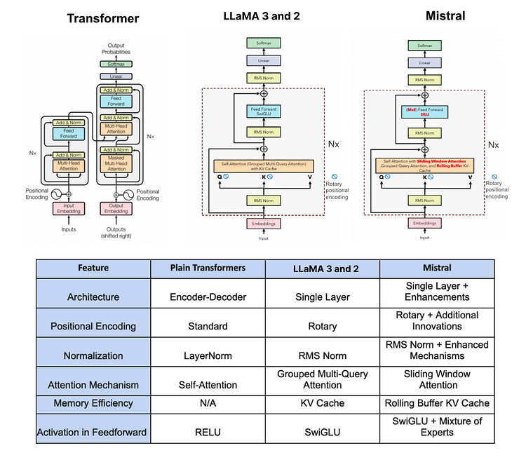
2. Tìm hiểu kiến ​​trúc Transformer của LLaMA 3

Hiểu kiến ​​trúc của LLaMA 3 là điều quan trọng trước khi đi sâu vào mã hóa nó. Để hiểu rõ hơn về hình ảnh, đây là sơ đồ so sánh giữa Transformer vani, LLaMA 2/3 và Mistral.

2.1. Pre-normalization bằng MSNorm

Trong phương pháp LLaMA 3, giống như LLaMA 2, có một kỹ thuật được gọi là RMSNorm được sử dụng để chuẩn hóa đầu vào của mỗi lớp con của transformer.

Hãy tưởng tượng bạn đang học cho một kỳ thi lớn, và bạn có một cuốn giáo trình khổng lồ với nhiều chương. Mỗi chương đại diện cho một chủ đề khác nhau, nhưng một số chương quan trọng hơn cho việc hiểu tổng thể môn học.

Trước khi đào sâu vào toàn bộ cuốn sách, bạn quyết định đánh giá tầm quan trọng của mỗi chương. Bạn không muốn dành cùng một lượng thời gian cho mỗi chương; bạn muốn tập trung nhiều hơn vào những chương quan trọng.

Đây là lúc Pre-normalization sử dụng RMSNorm xuất hiện trong các mô hình ngôn ngữ lớn (LLMs) như ChatGPT. Điều này giống như việc gán một trọng số cho mỗi chương dựa trên ý nghĩa của nó. Các chương cơ bản sẽ có trọng số cao hơn, trong khi những chương ít quan trọng hơn sẽ có trọng số thấp hơn.

Vì vậy, trước khi nghiên cứu sâu hơn, bạn điều chỉnh kế hoạch học dựa trên tầm quan trọng được gán cho từng chương. Bạn dành nhiều thời gian và nỗ lực hơn cho các chương có trọng số cao, đảm bảo bạn nắm vững các khái niệm cốt lõi.

Tương tự, việc sử dụng Pre-normalization với RMSNorm giúp các mô hình ngôn ngữ lớn ưu tiên các phần văn bản quan trọng hơn để hiểu rõ ngữ cảnh và ý nghĩa. Nó gán trọng số cao hơn cho các yếu tố cốt lõi và trọng số thấp hơn cho những yếu tố ít quan trọng, đảm bảo mô hình tập trung vào những nơi cần thiết nhất để hiểu một cách chính xác. Nếu bạn quan tâm đến cách triển khai chi tiết RMSNorm thì bạn có thể tìm hiểu thêm tại đây .

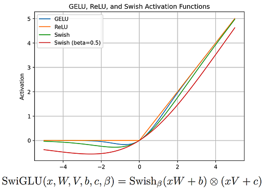
2.2. Hàm kích hoạt SwiGLU

SwiGLU (Swish-Gated Linear Unit) là một hàm kích hoạt mới kết hợp lợi ích của hàm kích hoạt Swish và đơn vị tuyến tính có cổng (GLU). Hàm kích hoạt này được đề xuất trong một bài báo của các nhà nghiên cứu tại Đại học Copenhagen vào năm 2019 và từ đó đã trở nên phổ biến trong cộng đồng học sâu.

Hãy tưởng tượng bạn là một giáo viên đang cố gắng giải thích một chủ đề phức tạp cho học sinh của mình. Bạn có một bảng trắng lớn để viết các điểm chính và vẽ sơ đồ để làm cho mọi thứ rõ ràng hơn. Tuy nhiên, đôi khi chữ viết của bạn có thể không gọn gàng lắm hoặc các sơ đồ của bạn có thể không được vẽ hoàn hảo. Điều này có thể làm cho việc hiểu nội dung trở nên khó khăn đối với học sinh.

Bây giờ, hãy tưởng tượng nếu bạn có một cây bút ma thuật có thể tự động điều chỉnh kích thước và kiểu chữ của chữ viết dựa trên tầm quan trọng của mỗi điểm. Nếu điều gì đó thực sự quan trọng, cây bút viết to hơn và rõ ràng hơn, làm cho nó nổi bật. Nếu nó không quan trọng bằng, cây bút viết nhỏ hơn, nhưng vẫn dễ đọc.

SwiGLU giống như cây bút ma thuật đó đối với các mô hình ngôn ngữ lớn (LLMs) như ChatGPT. Trước khi tạo văn bản, SwiGLU điều chỉnh tầm quan trọng của từng từ hoặc cụm từ dựa trên mức liên quan của chúng đối với ngữ cảnh. Giống như cây bút ma thuật điều chỉnh kích thước và kiểu chữ của bạn, SwiGLU điều chỉnh sự nhấn mạnh của từng từ hoặc cụm từ.

Vì vậy, khi mô hình ngôn ngữ lớn (LLM) tạo ra văn bản, nó có thể làm nổi bật các phần quan trọng hơn, làm cho chúng dễ nhận thấy hơn và đảm bảo chúng đóng góp nhiều hơn vào sự hiểu biết tổng thể của văn bản. Bằng cách này, SwiGLU giúp các LLM tạo ra văn bản rõ ràng và dễ hiểu hơn, giống như cách mà cây bút thần kỳ giúp bạn tạo ra những giải thích rõ ràng hơn cho học sinh trên bảng trắng. Thông tin chi tiết về SwiGLU có thể được tìm thấy trong bài báo liên quan.

2.3. Rotary Embeddings (RoPE)

Rotary Position Embedding (RoPE) là một loại nhúng vị trí được sử dụng trong LLaMA 3.

Hãy tưởng tượng bạn đang ở trong một lớp học và bạn muốn phân chia chỗ cho học sinh để tham gia vào các cuộc thảo luận nhóm. Thông thường, bạn có thể sắp xếp chỗ ngồi theo hàng và cột, với mỗi học sinh có một vị trí cố định. Tuy nhiên, trong một số trường hợp, bạn muốn tạo ra một sắp xếp chỗ ngồi linh hoạt hơn, cho phép học sinh di chuyển và tương tác tự do hơn.

RoPE giống như một sắp xếp chỗ ngồi đặc biệt, cho phép học sinh xoay vòng và thay đổi vị trí mà vẫn duy trì vị trí tương đối với nhau. Thay vì cố định ở một nơi, học sinh có thể di chuyển xung quanh theo hình tròn, tạo điều kiện cho các tương tác mượt mà hơn.

Trong tình huống này, mỗi học sinh đại diện cho một từ hoặc token trong một chuỗi văn bản, và vị trí của họ tương ứng với vị trí trong chuỗi. Giống như cách RoPE cho phép học sinh xoay vòng và thay đổi vị trí, RoPE cho phép nhúng vị trí của các từ trong một chuỗi văn bản thay đổi động dựa trên vị trí tương đối của chúng với nhau.

Vì vậy, khi xử lý văn bản, thay vì coi nhúng vị trí là cố định và tĩnh, RoPE giới thiệu khía cạnh xoay vòng, cho phép biểu diễn linh hoạt hơn để bắt kịp các mối quan hệ động giữa các từ trong chuỗi. Linh hoạt này giúp các mô hình như ChatGPT hiểu và tạo ra văn bản tự nhiên hơn và duy trì tính nhất quán, tương tự như cách sắp xếp chỗ ngồi động tạo điều kiện cho các cuộc thảo luận tương tác hơn trong lớp học. 

2.4. Thuật toán Byte Pair Encoding (BPE)

Trong LLaMA 3, việc sử dụng Byte Pair Encoding (BPE) được thực hiện từ thư viện tiktoken do OpenAI giới thiệu, trong khi tokenizer BPE của LLaMA 2 dựa trên thư viện sentencepiece. Có một sự khác biệt nhỏ giữa chúng, nhưng trước tiên, chúng ta hãy tìm hiểu BPE là gì.

Hãy bắt đầu với một ví dụ đơn giản. Giả sử chúng ta có một tập văn bản với các từ: “ab”, “bc”, “bcd” và “cde”. Chúng ta bắt đầu bằng cách khởi tạo từ vựng với tất cả các ký tự riêng lẻ trong tập văn bản, vì vậy từ vựng ban đầu của chúng ta là {“a”, “b”, “c”, “d”, “e”}.

Tiếp theo, chúng ta tính toán tần suất của mỗi ký tự trong tập văn bản. Đối với ví dụ của chúng ta, tần suất là: {“a”: 1, “b”: 3, “c”: 3, “d”: 2, “e”: 1}.

Bây giờ, chúng ta bắt đầu quá trình kết hợp. Chúng ta lặp lại các bước sau cho đến khi từ vựng đạt kích thước mong muốn:

• Đầu tiên, chúng ta tìm cặp ký tự liên tiếp phổ biến nhất. Trong trường hợp này, cặp phổ biến nhất là “bc” với tần suất là 2. Sau đó kết hợp cặp này để tạo ra một đơn vị con từ mới là “bc”. Sau khi kết hợp, chúng ta cập nhật lại tần suất để phản ánh đơn vị con từ mới. Tần suất đã cập nhật là {“a”: 1, “b”: 2, “c”: 2, “d”: 2, “e”: 1, “bc”: 2}. Chúng ta thêm đơn vị con từ mới “bc” vào từ vựng của chúng ta, từ đó trở thành {“a”, “b”, “c”, “d”, “e”, “bc”}. 

• Chúng ta lặp lại quá trình. Cặp tiếp theo phổ biến nhất là “cd”. Chúng ta kết hợp “cd” để tạo ra đơn vị con từ mới “cd” và cập nhật lại tần suất. Tần suất đã cập nhật là {“a”: 1, “b”: 2, “c”: 1, “d”: 1, “e”: 1, “bc”: 2, “cd”: 2}. Chúng ta thêm “cd” vào từ vựng, kết quả là {“a”, “b”, “c”, “d”, “e”, “bc”, “cd”}. 

• Tiếp tục quá trình, cặp phổ biến tiếp theo là “de”. Chúng ta kết hợp “de” để tạo ra đơn vị con từ “de” và cập nhật lại tần suất để {“a”: 1, “b”: 2, “c”: 1, “d”: 1, “e”: 0, “bc”: 2, “cd”: 1, “de”: 1}. Chúng ta thêm “de” vào từ vựng, tạo thành {“a”, “b”, “c”, “d”, “e”, “bc”, “cd”, “de”}. 

• Tiếp theo, chúng ta tìm “ab” là cặp phổ biến nhất. Chúng ta kết hợp “ab” để tạo ra đơn vị con từ “ab” và cập nhật lại tần suất để {“a”: 0, “b”: 1, “c”: 1, “d”: 1, “e”: 0, “bc”: 2, “cd”: 1, “de”: 1, “ab”: 1}. Chúng ta thêm “ab” vào từ vựng, từ đó trở thành {“a”, “b”, “c”, “d”, “e”, “bc”, “cd”, “de”, “ab”}. 

• Cặp phổ biến tiếp theo là “bcd”. Chúng ta kết hợp “bcd” để tạo ra đơn vị con từ “bcd” và cập nhật lại tần suất để {“a”: 0, “b”: 0, “c”: 0, “d”: 0, “e”: 0, “bc”: 1, “cd”: 0, “de”: 1, “ab”: 1, “bcd”: 1}. Chúng ta thêm “bcd” vào từ vựng, kết quả là {“a”, “b”, “c”, “d”, “e”, “bc”, “cd”, “de”, “ab”, “bcd”}. 

• Cuối cùng, cặp phổ biến nhất là “cde”. Chúng ta kết hợp “cde” để tạo ra đơn vị con từ “cde” và cập nhật lại tần suất để {“a”: 0, “b”: 0, “c”: 0, “d”: 0, “e”: 0, “bc”: 1, “cd”: 0, “de”: 0, “ab”: 1, “bcd”: 1, “cde”: 1}. Chúng ta thêm “cde” vào từ vựng, tạo thành {“a”, “b”, “c”, “d”, “e”, “bc”, “cd”, “de”, “ab”, “bcd”, “cde”}.

Phương pháp này có thể cải thiện hiệu suất của các mô hình ngôn ngữ lớn (LLMs) và xử lý các từ hiếm và không có trong từ vựng. Sự khác biệt lớn giữa TikToken BPE và sentencepiece BPE là TikToken BPE không chia các từ thành các phần nhỏ nếu toàn bộ từ đã được biết đến. Ví dụ, nếu từ “hugging” đã có trong từ vựng, nó sẽ được giữ lại làm một token thay vì chia thành [“hug”,”ging”]

3. Thiết lập cơ sở

Chúng ta sẽ làm việc với một loạt thư viện Python nhỏ, để tránh lỗi “no module found” tốt hơn hết bạn nên cài đặt tất cả chúng với lệnh sau:

pip install sentencepiece tiktoken torch blobfile matplotlib huggingface_hub

Sau khi cài đặt các thư viện cần thiết, chúng ta cần tải xuống một số tệp tin. Vì chúng ta sẽ sao chép kiến ​​trúc của llama-3–8B, bạn cần có một tài khoản trên HuggingFace. Ngoài ra, vì llama-3 là một mô hình có điều khiển, bạn phải chấp nhận các điều khoản và điều kiện của họ để truy cập nội dung mô hình.

Dưới đây là các bước:

• Tạo tài khoản trên HuggingFace.

• Chấp nhận các điều khoản và điều kiện của llama-3–8B.

Sau khi hoàn thành cả hai bước này, bây giờ chúng ta cần tải xuống một số tệp tin. Có hai lựa chọn để làm điều này:

Lựa chọn 1: Thủ công - Đi đến thư mục llama-3–8B trên HuggingFace từ liên kết này và tải xuống từng tệp tin sau:

Lựa chọn 2: Coding - Chúng ta có thể sử dụng thư viện hugging_face, đã được cài đặt trước đó, để tải xuống tất cả các tệp tin này. Tuy nhiên, trước tiên, chúng ta cần đăng nhập vào HuggingFace Hub trong sổ tay làm việc của chúng ta bằng HF Token của chúng ta. Bạn có thể tạo một mã token mới hoặc truy cập tại đây.

# Import the `notebook_login` function from the `huggingface_hub` module.
from huggingface_hub import notebook_login

# Execute the `notebook_login` function to log in to the Hugging Face Hub.
notebook_login()

Sau khi bạn chạy lệnh này, nó sẽ yêu cầu bạn nhập mã token. Nếu có lỗi khi đăng nhập, hãy thử lại nhưng hãy bỏ tùy chọn "add token as git credential". Sau đó, chúng ta chỉ cần chạy một đoạn mã Python đơn giản để tải xuống ba tệp tin là cốt lõi của kiến trúc llama-3–8B.

# Import the necessary function from the huggingface_hub library
from huggingface_hub import hf_hub_download

# Define the repository information
repo_id = "meta-llama/Meta-Llama-3-8B"
subfolder = "original" # Specify the subfolder within the repository

# List of filenames to download
filenames = ["params.json", "tokenizer.model", "consolidated.00.pth"]

# Specify the directory where you want to save the downloaded files
save_directory = "llama-3-8B/" # Replace with your desired path

# Download each file
for filename in filenames:
hf_hub_download(
repo_id=repo_id, # Repository ID
filename=filename, # Name of the file to download
subfolder=subfolder, # Subfolder within the repository
local_dir=save_directory # Directory to save the downloaded file
)

Sau khi tải xuống tất cả các tệp tin, chúng ta cần nhập các thư viện mà chúng ta sẽ sử dụng.

# Tokenization library
import tiktoken

# BPE loading function
from tiktoken.load import load_tiktoken_bpe

# PyTorch library
import torch

# JSON handling
import json

4. Hiểu cấu trúc tệp

Chúng ta đang nhắm đến việc sao chép chính xác kiến trúc của llama-3, điều này đồng nghĩa với việc văn bản đầu vào của chúng ta phải cho ra một kết quả có ý nghĩa. Ví dụ, nếu văn bản đầu vào của chúng ta là “màu của mặt trời là gì?”, thì kết quả phải là “trắng”. Để đạt được điều này, chúng ta cần huấn luyện mô hình ngôn ngữ trên một tập dữ liệu lớn, đòi hỏi khả năng tính toán cao, làm cho việc này trở nên không khả thi đối với chúng ta.

Tuy nhiên, Meta đã công khai phát hành các tệp kiến trúc của llama-3, hoặc theo cách phức tạp hơn, các trọng số đã được huấn luyện, để sử dụng. Chúng ta vừa tải xuống những tệp này, cho phép chúng ta sao chép kiến trúc của họ mà không cần huấn luyện hoặc một tập dữ liệu lớn. Mọi thứ đã được chuẩn bị sẵn, chúng ta chỉ cần sử dụng các thành phần phù hợp vào đúng vị trí.

Hãy xem xét từng tệp và tầm quan trọng của chúng:

• tokenizer.model: Như chúng ta đã thảo luận trước đó, LLaMA-3 sử dụng tokenizer Byte Pair Encoding (BPE) từ tiktoken, được huấn luyện trên một tập dữ liệu có 15 nghìn tỷ token — lớn gấp 7 lần so với tập dữ liệu được sử dụng cho LLaMA-2. Hãy tải tệp này lên và xem nó chứa gì

# Loading the tokenizer from llama-3-8B
tokenizer_model = load_tiktoken_bpe("tokenizer.model")

# Get the length of the tokenizer model
len(tokenizer_model)
# OUTPUT: 128000

# Get the type of the `tokenizer_model` object.
type(tokenizer_model)
# OUTPUT: dictionary

Thuộc tính length hiển thị kích thước từ vựng tổng cộng, đó là số lượng duy nhất các ký tự trong dữ liệu huấn luyện. Kiểu dữ liệu của tokenizer_model là một từ điển (dictionary).

# Printing the first 10 items of tokenizer model
dict(list(tokenizer_model.items())[5600:5610])

#### OUTPUT ####
{

b'mitted': 5600,
b" $('#": 5601,
b' saw': 5602,
b' approach': 5603,
b'ICE': 5604,
b' saying': 5605,
b' anyone': 5606,
b'meta': 5607,
b'SD': 5608,
b' song': 5609

}
#### OUTPUT ####

Nếu chúng ta in 10 mục (item) ngẫu nhiên từ tệp này, bạn sẽ thấy các chuỗi ký tự được tạo thành bằng thuật toán BPE, giống như ví dụ chúng ta đã thảo luận trước đó. Trong tệp, các khóa đại diện cho chuỗi byte từ quá trình huấn luyện BPE, còn giá trị đại diện cho thứ hạng hợp nhất dựa trên tần suất xuất hiện. 

• consolidated.00.pth chứa các tham số đã học được (trọng số) của Llama-3B-8B. Các tham số này bao gồm thông tin về cách mô hình hiểu và xử lý ngôn ngữ, chẳng hạn như cách nó biểu diễn các token (đơn vị từ ngữ), tính toán chú ý (attention), thực hiện các phép biến đổi feed-forward và chuẩn hóa đầu ra.

# Loading a PyTorch model of LLaMA-3-8B
model = torch.load("consolidated.00.pth")

# printing first 11 layers of the architecture
list(model.keys())[:11]

#### OUTPUT ####
[

'tok_embeddings.weight',
'layers.0.attention.wq.weight',
'layers.0.attention.wk.weight',
'layers.0.attention.wv.weight',
'layers.0.attention.wo.weight',
'layers.0.feed_forward.w1.weight',
'layers.0.feed_forward.w3.weight',
'layers.0.feed_forward.w2.weight',
'layers.0.attention_norm.weight',
'layers.0.ffn_norm.weight',
'layers.1.attention.wq.weight',

]
#### OUTPUT ####

Nếu bạn quen thuộc với kiến ​​trúc transformer, bạn sẽ biết về truy vấn, ma trận khóa, v.v. Sau này, chúng ta sẽ sử dụng các lớp/trọng số này để tạo các ma trận như vậy trong kiến ​​trúc của Llama-3.

• params.json— chứa nhiều giá trị tham số khác nhau, chẳng hạn như:

# Opening the parameters JSON file
with open("params.json", "r") as f:
config = json.load(f)

# Printing the content
print(config)

#### OUTPUT ####
{

'dim': 4096,
'n_layers': 32,
'n_heads': 32,
'n_kv_heads': 8,
'vocab_size': 128256,
'multiple_of': 1024,
'ffn_dim_multiplier': 1.3,
'norm_eps': 1e-05,
'rope_theta': 500000.0

}
#### OUTPUT ####

Những giá trị này sẽ giúp chúng ta sao chép kiến trúc Llama-3 bằng cách chỉ định các chi tiết như số lượng heads, kích thước của vector nhúng và nhiều hơn nữa.

Hãy lưu trữ các giá trị này để chúng ta có thể sử dụng chúng sau này.

# Dimension
dim = config["dim"]

# Layers
n_layers = config["n_layers"]

# Heads
n_heads = config["n_heads"]

# KV_heads
n_kv_heads = config["n_kv_heads"]

# Vocabulary
vocab_size = config["vocab_size"]

# Multiple
multiple_of = config["multiple_of"]

# Multiplier
ffn_dim_multiplier = config["ffn_dim_multiplier"]

# Epsilon
norm_eps = config["norm_eps"]

# RoPE
rope_theta = torch.tensor(config["rope_theta"])

5. Token dữ liệu đầu vào

Điều đầu tiên cần thực hiện là chuyển đổi văn bản đầu vào thành các token, và để làm được điều này, chúng ta cần tạo ra một số token đặc biệt cần thiết để đưa ra các đánh dấu cấu trúc trong văn bản đã được mã hóa thành token, cho phép tokenizer nhận diện và xử lý các điều kiện hoặc hướng dẫn cụ thể.

special_tokens = [
"<|begin_of_text|>", # Marks the beginning of a text sequence.
"<|end_of_text|>", # Marks the end of a text sequence.
"<|reserved_special_token_0|>", # Reserved for future use.
"<|reserved_special_token_1|>", # Reserved for future use.
"<|reserved_special_token_2|>", # Reserved for future use.
"<|reserved_special_token_3|>", # Reserved for future use.
"<|start_header_id|>", # Indicates the start of a header ID.
"<|end_header_id|>", # Indicates the end of a header ID.
"<|reserved_special_token_4|>", # Reserved for future use.
"<|eot_id|>", # Marks the end of a turn (in a conversational context).
] + [f"<|reserved_special_token_{i}|>" for i in range(5, 256 - 5)] # A large set of tokens reserved for future use.

Tiếp theo, chúng ta sẽ định nghĩa các quy tắc để chia văn bản thành các token bằng cách xác định các mẫu khác nhau để phù hợp với các loại chuỗi con khác trong văn bản đầu vào. Đây là cách chúng ta có thể làm điều đó.

# patterns based on which text will be break into tokens
tokenize_breaker = r"(?i:'s|'t|'re|'ve|'m|'ll|'d)|[^\r\n\p{L}\p{N}]?\p{L}+|\p{N}{1,3}| ?[^\s\p{L}\p{N}]+[\r\n]*|\s*[\r\n]+|\s+(?!\S)|\s+"

Đoạn code trên có thể trích xuất từ, rút gọn, số (lên đến ba chữ số), và các chuỗi các ký tự không phải là khoảng trắng từ văn bản đầu vào, bạn có thể tùy chỉnh nó dựa trên yêu cầu của bạn.

Chúng ta cần viết một hàm mã hóa/giải mã mã thông báo đơn giản sử dụng TikToken BPE, với ba đối số: tokenizer_model, tokenize_breaker và special_tokens. Hàm này sẽ mã hóa/giải mã văn bản đầu vào của chúng ta tương ứng.

# Initialize tokenizer with specified parameters
tokenizer = tiktoken.Encoding(

# make sure to set path to tokenizer.model file
name = "tokenizer.model",

# Define tokenization pattern string
pat_str = tokenize_breaker,

# Assign BPE mergeable ranks from tokenizer_model of LLaMA-3
mergeable_ranks = tokenizer_model,

# Set special tokens with indices
special_tokens={token: len(tokenizer_model) + i for i, token in enumerate(special_tokens)},
)

# Encode "hello world!" and decode tokens to string
tokenizer.decode(tokenizer.encode("hello world!"))

#### OUTPUT ####
hello world!
#### OUTPUT ####

Để xác minh rằng các phương pháp của chúng ta trong hàm mã hóa hoạt động đúng, chúng ta sẽ truyền chuỗi “Hello World” vào hàm. Đầu tiên, nó sẽ mã hóa văn bản đó, biến nó thành các giá trị số. Sau đó, nó sẽ giải mã trở lại thành văn bản, kết quả là "hello world!". Điều này xác nhận rằng hàm đang hoạt động đúng đắn. Tiếp theo chúng ta sẽ token dữ liệu đầu vào

# input prompt
prompt = "the answer to the ultimate question of life, the universe, and everything is "

# Encode the prompt using the tokenizer and prepend a special token (128000)
tokens = [128000] + tokenizer.encode(prompt)

print(tokens) # Print the encoded tokens

# Convert the list of tokens into a PyTorch tensor
tokens = torch.tensor(tokens)

# Decode each token back into its corresponding string
prompt_split_as_tokens = [tokenizer.decode([token.item()]) for token in tokens]

print(prompt_split_as_tokens) # Print the decoded tokens


#### OUTPUT ####
[128000, 1820, 4320, 311, ... ]
['<|begin_of_text|>', 'the', ' answer', ' to', ... ]
#### OUTPUT ####

6. Tạo Embedding cho mỗi Token

Nếu chúng ta check vector đầu vào thì nó sẽ như thế sau:

# checking dimension of input vector
len(tokens)

#### OUTPUT ####
17
#### OUTPUT ####

# checking dimension of embedding vector from llama-3 architecture
print(dim)

#### OUTPUT ####
4096
#### OUTPUT ####

Chúng ta cần biến đổi các vectơ đầu vào của chúng ta (hiện tại có kích thước (17x1)) thành embedding cho mỗi từ đã được phân đoạn. Điều này có nghĩa là các token (17x1) của chúng ta sẽ trở thành (17x4096), trong đó mỗi token sẽ có một embedding tương ứng có chiều dài 4096.

# Define embedding layer with vocab size and embedding dimension
embedding_layer = torch.nn.Embedding(vocab_size, dim)

# Copy pre-trained token embeddings to the embedding layer
embedding_layer.weight.data.copy_(model["tok_embeddings.weight"])

# Get token embeddings for given tokens, converting to torch.bfloat16 format
token_embeddings_unnormalized = embedding_layer(tokens).to(torch.bfloat16)

# Print shape of resulting token embeddings
token_embeddings_unnormalized.shape


#### OUTPUT ####
torch.Size([17, 4096])
#### OUTPUT ####

Các embedding này chưa được chuẩn hóa, và nếu chúng ta không chuẩn hóa chúng, sẽ có tác động nghiêm trọng. Trong phần tiếp theo, chúng ta sẽ thực hiện chuẩn hóa trên các vectơ đầu vào. 

7. Chuẩn hóa bằng RMSNorm

Chúng ta sẽ chuẩn hóa các vector đầu vào bằng cách sử dụng công thức như chúng ta đã thấy trước đó cho RMSNorm

# Calculating RMSNorm
def rms_norm(tensor, norm_weights):

# Calculate the mean of the square of tensor values along the last dimension
squared_mean = tensor.pow(2).mean(-1, keepdim=True)

# Add a small value to avoid division by zero
normalized = torch.rsqrt(squared_mean + norm_eps)

# Multiply normalized tensor by the provided normalization weights
return (tensor * normalized) * norm_weights

Để chuẩn hóa các embedding chưa được chuẩn hóa, chúng ta có thể sử dụng trọng số chú ý từ layers_0. Lý do sử dụng layer_0 là vì chúng ta đang tạo lớp đầu tiên của kiến trúc transformer LLaMA-3.

# using RMS normalization and provided normalization weights
token_embeddings = rms_norm(token_embeddings_unnormalized,
model["layers.0.attention_norm.weight"])

# Print the shape of the resulting token embeddings
token_embeddings.shape


#### OUTPUT ####
torch.Size([17, 4096])
#### OUTPUT ####

8. Attention Heads (Query, Key, Values)

Đầu tiên, hãy load các query, key, value và output vectors từ mô hình. 

# Print the shapes of different weights
print(
# Query weight shape
model["layers.0.attention.wq.weight"].shape,

# Key weight shape
model["layers.0.attention.wk.weight"].shape,

# Value weight shape
model["layers.0.attention.wv.weight"].shape,

# Output weight shape
model["layers.0.attention.wo.weight"].shape
)


#### OUTPUT ####
torch.Size([4096, 4096]) # Query weight dimension
torch.Size([1024, 4096]) # Key weight dimension
torch.Size([1024, 4096]) # Value weight dimension
torch.Size([4096, 4096]) # Output weight dimension
#### OUTPUT ####

Kích thước này cho thấy rằng các trọng số mô hình mà chúng ta đã tải xuống không phải cho từng head riêng lẻ mà cho nhiều head atention do việc thực hiện một phương pháp/đào tạo song song. Tuy nhiên, chúng ta có thể “mở” những ma trận này để chỉ sử dụng cho một head duy nhất.

# Retrieve query weight for the first layer of attention
q_layer0 = model["layers.0.attention.wq.weight"]

# Calculate dimension per head
head_dim = q_layer0.shape[0] // n_heads

# Reshape query weight to separate heads
q_layer0 = q_layer0.view(n_heads, head_dim, dim)

# Print the shape of the reshaped query weight tensor
q_layer0.shape


#### OUTPUT ####
torch.Size([32, 128, 4096])
#### OUTPUT ####

Ở đây, 32 là số lượng head của attention mechanism trong Llama-3, 128 là kích thước của vector query, và 4096 là kích thước của embedding token.

Chúng ta có thể truy cập ma trận weight của query thuộc head đầu tiên ở lớp đầu tiên bằng cách sử dụng lệnh:

# Extract the query weight for the first head of the first layer of attention
q_layer0_head0 = q_layer0[0]

# Print the shape of the extracted query weight tensor for the first head
q_layer0_head0.shape


#### OUTPUT ####
torch.Size([128, 4096])
#### OUTPUT ####

Để tìm vector query cho mỗi token, chúng ta thực hiện phép nhân giữa ma trận weight của query với embedding token.

# Matrix multiplication: token embeddings with transpose of query weight for first head
q_per_token = torch.matmul(token_embeddings, q_layer0_head0.T)

# Shape of resulting tensor: queries per token
q_per_token.shape


#### OUTPUT ####
torch.Size([17, 128])
#### OUTPUT ####

Các vector query theo mặc định không tự biết vị trí của chúng trong đoạn văn (prompt) ban đầu. Do đó, chúng ta sẽ sử dụng RoPE để cung cấp thông tin về vị trí cho chúng.

9. Triển khai RoPE

Chúng ta chia các vector query thành từng cặp và sau đó áp dụng phép dịch chuyển góc xoay cho từng cặp.

# Convert queries per token to float and split into pairs
q_per_token_split_into_pairs = q_per_token.float().view(q_per_token.shape[0], -1, 2)

# Print the shape of the resulting tensor after splitting into pairs
q_per_token_split_into_pairs.shape


#### OUTPUT ####
torch.Size([17, 64, 2])
#### OUTPUT ####

Chúng ta có một vector kích thước [17x64x2], đại diện cho các truy vấn ban đầu có độ dài 128 được chia thành 64 cặp cho mỗi token trong đoạn văn. Mỗi cặp sẽ được xoay một góc m*theta, trong đó m là vị trí của token mà chúng ta đang xoay vector query. Chúng ta sẽ sử dụng tích vô hướng của số phức để xoay một vectơ.

# Generate values from 0 to 1 split into 64 parts
zero_to_one_split_into_64_parts = torch.tensor(range(64))/64

# Print the resulting tensor
zero_to_one_split_into_64_parts


#### OUTPUT ####
tensor([0.0000, 0.0156, 0.0312, 0.0469, 0.0625, 0.0781, 0.0938, 0.1094, 0.1250,
0.1406, 0.1562, 0.1719, 0.1875, 0.2031, 0.2188, 0.2344, 0.2500, 0.2656,
0.2812, 0.2969, 0.3125, 0.3281, 0.3438, 0.3594, 0.3750, 0.3906, 0.4062,
0.4219, 0.4375, 0.4531, 0.4688, 0.4844, 0.5000, 0.5156, 0.5312, 0.5469,
0.5625, 0.5781, 0.5938, 0.6094, 0.6250, 0.6406, 0.6562, 0.6719, 0.6875,
0.7031, 0.7188, 0.7344, 0.7500, 0.7656, 0.7812, 0.7969, 0.8125, 0.8281,
0.8438, 0.8594, 0.8750, 0.8906, 0.9062, 0.9219, 0.9375, 0.9531, 0.9688,
0.9844])
#### OUTPUT ####

Sau bước tách chúng ta sẽ tính tần số của nó.

# Calculate frequencies using a power operation
freqs = 1.0 / (rope_theta ** zero_to_one_split_into_64_parts)

# Display the resulting frequencies
freqs


#### OUTPUT ####
tensor([1.0000e+00, 8.1462e-01, 6.6360e-01, 5.4058e-01, 4.4037e-01, 3.5873e-01,
2.9223e-01, 2.3805e-01, 1.9392e-01, 1.5797e-01, 1.2869e-01, 1.0483e-01,
8.5397e-02, 6.9566e-02, 5.6670e-02, 4.6164e-02, 3.7606e-02, 3.0635e-02,
2.4955e-02, 2.0329e-02, 1.6560e-02, 1.3490e-02, 1.0990e-02, 8.9523e-03,
7.2927e-03, 5.9407e-03, 4.8394e-03, 3.9423e-03, 3.2114e-03, 2.6161e-03,
2.1311e-03, 1.7360e-03, 1.4142e-03, 1.1520e-03, 9.3847e-04, 7.6450e-04,
6.2277e-04, 5.0732e-04, 4.1327e-04, 3.3666e-04, 2.7425e-04, 2.2341e-04,
1.8199e-04, 1.4825e-04, 1.2077e-04, 9.8381e-05, 8.0143e-05, 6.5286e-05,
5.3183e-05, 4.3324e-05, 3.5292e-05, 2.8750e-05, 2.3420e-05, 1.9078e-05,
1.5542e-05, 1.2660e-05, 1.0313e-05, 8.4015e-06, 6.8440e-06, 5.5752e-06,
4.5417e-06, 3.6997e-06, 3.0139e-06, 2.4551e-06])
#### OUTPUT ####

Bây giờ, với một số phức cho mỗi phần tử truy vấn của token, chúng ta chuyển đổi các truy vấn của chúng ta thành số phức và sau đó xoay chúng dựa trên vị trí của chúng bằng cách sử dụng tích vô hướng.

# Convert queries per token to complex numbers
q_per_token_as_complex_numbers = torch.view_as_complex(q_per_token_split_into_pairs)

q_per_token_as_complex_numbers.shape
# Output: torch.Size([17, 64])

# Calculate frequencies for each token using outer product of arange(17) and freqs
freqs_for_each_token = torch.outer(torch.arange(17), freqs)

# Calculate complex numbers from frequencies_for_each_token using polar coordinates
freqs_cis = torch.polar(torch.ones_like(freqs_for_each_token), freqs_for_each_token)

# Rotate complex numbers by frequencies
q_per_token_as_complex_numbers_rotated = q_per_token_as_complex_numbers * freqs_cis

q_per_token_as_complex_numbers_rotated.shape
# Output: torch.Size([17, 64])

Sau khi thu được vector đã xoay, chúng ta có thể chuyển đổi chúng về lại dạng truy vấn gốc theo cặp bằng cách xem lại các số phức như các số thực.

# Convert rotated complex numbers back to real numbers
q_per_token_split_into_pairs_rotated = torch.view_as_real(q_per_token_as_complex_numbers_rotated)

# Print the shape of the resulting tensor
q_per_token_split_into_pairs_rotated.shape


#### OUTPUT ####
torch.Size([17, 64, 2])
#### OUTPUT ####

Các cặp đã xoay hiện được merge, tạo ra một vectơ truy vấn mới có hình dạng [17x128], trong đó 17 là số lượng token và 128 là kích thước của vectơ truy vấn.

# Reshape rotated token queries to match the original shape
q_per_token_rotated = q_per_token_split_into_pairs_rotated.view(q_per_token.shape)

# Print the shape of the resulting tensor
q_per_token_rotated.shape


#### OUTPUT ####
torch.Size([17, 128])
#### OUTPUT ####

Quá trình xử lý key (khóa) tương tự như với query (ph truy vấn), nhưng cần lưu ý rằng vector key cũng có kích thước 128 chiều. Số lượng weight của key chỉ bằng 1/4 so với query vì chúng được chia sẻ giữa 4 head cùng một lúc để giảm thiểu tính toán. Key cũng được xoay để bao gồm thông tin về vị trí, giống như query.

# Extract the weight tensor for the attention mechanism's key in the first layer of the model
k_layer0 = model["layers.0.attention.wk.weight"]

# Reshape key weight for the first layer of attention to separate heads
k_layer0 = k_layer0.view(n_kv_heads, k_layer0.shape[0] // n_kv_heads, dim)

# Print the shape of the reshaped key weight tensor
k_layer0.shape # Output: torch.Size([8, 128, 4096])

# Extract the key weight for the first head of the first layer of attention
k_layer0_head0 = k_layer0[0]

# Print the shape of the extracted key weight tensor for the first head
k_layer0_head0.shape # Output: torch.Size([128, 4096])

# Calculate key per token by matrix multiplication
k_per_token = torch.matmul(token_embeddings, k_layer0_head0.T)

# Print the shape of the resulting tensor representing keys per token
k_per_token.shape # Output: torch.Size([17, 128])

# Split key per token into pairs and convert to float
k_per_token_split_into_pairs = k_per_token.float().view(k_per_token.shape[0], -1, 2)

# Print the shape of the resulting tensor after splitting into pairs
k_per_token_split_into_pairs.shape # Output: torch.Size([17, 64, 2])

# Convert key per token to complex numbers
k_per_token_as_complex_numbers = torch.view_as_complex(k_per_token_split_into_pairs)

# Print the shape of the resulting tensor representing key per token as complex numbers
k_per_token_as_complex_numbers.shape # Output: torch.Size([17, 64])

# Rotate complex key per token by frequencies
k_per_token_split_into_pairs_rotated = torch.view_as_real(k_per_token_as_complex_numbers * freqs_cis)

# Print the shape of the rotated complex key per token
k_per_token_split_into_pairs_rotated.shape # Output: torch.Size([17, 64, 2])

# Reshape rotated key per token to match the original shape
k_per_token_rotated = k_per_token_split_into_pairs_rotated.view(k_per_token.shape)

# Print the shape of the rotated key per token
k_per_token_rotated.shape # Output: torch.Size([17, 128])

Bây giờ chúng ta có các query và key đã được xoay cho mỗi token, với kích thước của mỗi thành phần đều là [17x128]

10. Triển khai Self Attention

Việc nhân ma trận query và key sẽ cung cấp cho chúng ta một điểm số, điểm số này ánh xạ mỗi token (ký hiệu) sang một token khác. Điều này biểu thị cho mức độ liên quan giữa query và key của từng token.

# Calculate query-key dot products per token
qk_per_token = torch.matmul(q_per_token_rotated, k_per_token_rotated.T) / (head_dim) ** 0.5

# Print the shape of the resulting tensor representing query-key dot products per token
qk_per_token.shape


#### OUTPUT ####
torch.Size([17, 17])
#### OUTPUT ####

Kích thước [17x17] biểu diễn điểm chú ý (attention score) (ký hiệu qk_per_token), trong đó 17 là số lượng token trong đoạn văn.

Chúng ta cần che các điểm giữa query-key. Trong quá trình huấn luyện, điểm giữa các query-key của các token tương lai sẽ bị che bởi vì mô hình chỉ học dự đoán các token dựa trên các token đã xuất hiện trước đó. Do đó, trong quá trình suy luận, chúng ta đặt các điểm tương ứng với các token tương lai về 0.

# Create a mask tensor filled with negative infinity values
mask = torch.full((len(tokens), len(tokens)), float("-inf"), device=tokens.device)

# Set upper triangular part of the mask tensor to negative infinity
mask = torch.triu(mask, diagonal=1)

# Print the resulting mask tensor
mask


#### OUTPUT ####
tensor([[0., -inf, -inf, -inf, -inf, -inf, -inf, -inf, -inf, -inf, -inf, -inf, -inf, -inf, -inf, -inf, -inf],
[0., 0., -inf, -inf, -inf, -inf, -inf, -inf, -inf, -inf, -inf, -inf, -inf, -inf, -inf, -inf, -inf],
[0., 0., 0., -inf, -inf, -inf, -inf, -inf, -inf, -inf, -inf, -inf, -inf, -inf, -inf, -inf, -inf],
[0., 0., 0., 0., -inf, -inf, -inf, -inf, -inf, -inf, -inf, -inf, -inf, -inf, -inf, -inf, -inf],
[0., 0., 0., 0., 0., -inf, -inf, -inf, -inf, -inf, -inf, -inf, -inf, -inf, -inf, -inf, -inf],
[0., 0., 0., 0., 0., 0., -inf, -inf, -inf, -inf, -inf, -inf, -inf, -inf, -inf, -inf, -inf],
[0., 0., 0., 0., 0., 0., 0., -inf, -inf, -inf, -inf, -inf, -inf, -inf, -inf, -inf, -inf],
[0., 0., 0., 0., 0., 0., 0., 0., -inf, -inf, -inf, -inf, -inf, -inf, -inf, -inf, -inf],
[0., 0., 0., 0., 0., 0., 0., 0., 0., -inf, -inf, -inf, -inf, -inf, -inf, -inf, -inf],
[0., 0., 0., 0., 0., 0., 0., 0., 0., 0., -inf, -inf, -inf, -inf, -inf, -inf, -inf],
[0., 0., 0., 0., 0., 0., 0., 0., 0., 0., 0., -inf, -inf, -inf, -inf, -inf, -inf],
[0., 0., 0., 0., 0., 0., 0., 0., 0., 0., 0., 0., -inf, -inf, -inf, -inf, -inf],
[0., 0., 0., 0., 0., 0., 0., 0., 0., 0., 0., 0., 0., -inf, -inf, -inf, -inf],
[0., 0., 0., 0., 0., 0., 0., 0., 0., 0., 0., 0., 0., 0., -inf, -inf, -inf],
[0., 0., 0., 0., 0., 0., 0., 0., 0., 0., 0., 0., 0., 0., 0., -inf, -inf],
[0., 0., 0., 0., 0., 0., 0., 0., 0., 0., 0., 0., 0., 0., 0., 0., -inf],
[0., 0., 0., 0., 0., 0., 0., 0., 0., 0., 0., 0., 0., 0., 0., 0., 0.]])
#### OUTPUT ####

Bây giờ, chúng ta cần áp dụng mask lên vector điểm chú ý giữa query-key của mỗi token. Ngoài ra, chúng ta muốn áp dụng hàm softmax lên kết quả này để chuyển các điểm số đầu ra thành xác suất. Điều này giúp ích trong việc lựa chọn token hoặc chuỗi token có khả năng xuất hiện cao nhất từ vốn từ của mô hình, làm cho dự đoán của mô hình dễ hiểu hơn và phù hợp cho các tác vụ như tạo văn bản và phân loại văn bản.

# Add the mask to the query-key dot products per token
qk_per_token_after_masking = qk_per_token + mask

# Apply softmax along the second dimension after masking
qk_per_token_after_masking_after_softmax = torch.nn.functional.softmax(qk_per_token_after_masking, dim=1).to(torch.bfloat16)

Đối với ma trận giá trị (value matrix), đánh dấu phần kết thúc của quá trình self-attention, tương tự như ma trận key, các weight của giá trị cũng được chia sẻ trên 4 attention head để tiết kiệm tính toán. Kết quả là, kích thước của ma trận weight giá trị là [8x128x4096].

# Retrieve the value weight for the first layer of attention
v_layer0 = model["layers.0.attention.wv.weight"]

# Reshape value weight for the first layer of attention to separate heads
v_layer0 = v_layer0.view(n_kv_heads, v_layer0.shape[0] // n_kv_heads, dim)

# Print the shape of the reshaped value weight tensor
v_layer0.shape


#### OUTPUT ####
torch.Size([8, 128, 4096])
#### OUTPUT ####

Tương tự như các ma trận truy vấn và khóa, ma trận giá trị cho lớp đầu tiên và head đầu tiên có thể được lấy bằng cách sử dụng:

# Extract the value weight for the first head of the first layer of attention
v_layer0_head0 = v_layer0[0]

# Print the shape of the extracted value weight tensor for the first head
v_layer0_head0.shape


#### OUTPUT ####
torch.Size([128, 4096])
#### OUTPUT ####

Sử dụng trọng số giá trị, chúng ta tính toán các giá trị chú ý cho mỗi token, dẫn đến một ma trận có kích thước [17x128]. Ở đây, 17 biểu thị số lượng token trong prompt, và 128 chỉ ra kích thước của vector giá trị cho mỗi token.

# Calculate value per token by matrix multiplication
v_per_token = torch.matmul(token_embeddings, v_layer0_head0.T)

# Print the shape of the resulting tensor representing values per token
v_per_token.shape


#### OUTPUT ####
torch.Size([17, 128])
#### OUTPUT ####

Để có được ma trận chú ý kết quả (resulting attention matrix), chúng ta có thể thực hiện phép nhân sau:

# Calculate QKV attention by matrix multiplication
qkv_attention = torch.matmul(qk_per_token_after_masking_after_softmax, v_per_token)

# Print the shape of the resulting tensor
qkv_attention.shape


#### OUTPUT ####
torch.Size([17, 128])
#### OUTPUT ####

11. Triển khai Multi-Head Attention

Một vòng lặp sẽ được thực thi để thực hiện các phép tính giống như trên, nhưng cho mỗi head trong lớp đầu tiên.

# Store QKV attention for each head in a list
qkv_attention_store = []

# Iterate through each head
for head in range(n_heads):
# Extract query, key, and value weights for the current head
q_layer0_head = q_layer0[head]
k_layer0_head = k_layer0[head//4] # Key weights are shared across 4 heads
v_layer0_head = v_layer0[head//4] # Value weights are shared across 4 heads

# Calculate query per token by matrix multiplication
q_per_token = torch.matmul(token_embeddings, q_layer0_head.T)

# Calculate key per token by matrix multiplication
k_per_token = torch.matmul(token_embeddings, k_layer0_head.T)

# Calculate value per token by matrix multiplication
v_per_token = torch.matmul(token_embeddings, v_layer0_head.T)

# Split query per token into pairs and rotate them
q_per_token_split_into_pairs = q_per_token.float().view(q_per_token.shape[0], -1, 2)
q_per_token_as_complex_numbers = torch.view_as_complex(q_per_token_split_into_pairs)
q_per_token_split_into_pairs_rotated = torch.view_as_real(q_per_token_as_complex_numbers * freqs_cis[:len(tokens)])
q_per_token_rotated = q_per_token_split_into_pairs_rotated.view(q_per_token.shape)

# Split key per token into pairs and rotate them
k_per_token_split_into_pairs = k_per_token.float().view(k_per_token.shape[0], -1, 2)
k_per_token_as_complex_numbers = torch.view_as_complex(k_per_token_split_into_pairs)
k_per_token_split_into_pairs_rotated = torch.view_as_real(k_per_token_as_complex_numbers * freqs_cis[:len(tokens)])
k_per_token_rotated = k_per_token_split_into_pairs_rotated.view(k_per_token.shape)

# Calculate query-key dot products per token
qk_per_token = torch.matmul(q_per_token_rotated, k_per_token_rotated.T) / (128) ** 0.5

# Create a mask tensor filled with negative infinity values
mask = torch.full((len(tokens), len(tokens)), float("-inf"), device=tokens.device)
# Set upper triangular part of the mask tensor to negative infinity
mask = torch.triu(mask, diagonal=1)
# Add the mask to the query-key dot products per token
qk_per_token_after_masking = qk_per_token + mask

# Apply softmax along the second dimension after masking
qk_per_token_after_masking_after_softmax = torch.nn.functional.softmax(qk_per_token_after_masking, dim=1).to(torch.bfloat16)

# Calculate QKV attention by matrix multiplication
qkv_attention = torch.matmul(qk_per_token_after_masking_after_softmax, v_per_token)

# Store QKV attention for the current head
qkv_attention_store.append(qkv_attention)

# Print the number of QKV attentions stored
len(qkv_attention_store)


#### OUTPUT ####
32
#### OUTPUT ####

Bây giờ, sau khi có được ma trận chú ý QKV cho tất cả 32 head trong lớp đầu tiên, tất cả các điểm chú ý sẽ được hợp nhất thành một ma trận lớn hơn có kích thước [17x4096].

# Concatenate QKV attentions from all heads along the last dimension
stacked_qkv_attention = torch.cat(qkv_attention_store, dim=-1)

# Print the shape of the resulting tensor
stacked_qkv_attention.shape


#### OUTPUT ####
torch.Size([17, 4096])
#### OUTPUT ####

Một trong những bước cuối cùng của tính toán Self-Attention trong lớp 0 là nhân ma trận weight với ma trận QKV đã xếp chồng (stacked QKV matrix).

# Calculate the embedding delta by matrix multiplication with the output weight
embedding_delta = torch.matmul(stacked_qkv_attention, model["layers.0.attention.wo.weight"].T)

# Print the shape of the resulting tensor
embedding_delta.shape


#### OUTPUT ####
torch.Size([17, 4096])
#### OUTPUT ####

Bây giờ, chúng ta đã có được sự thay đổi trong giá trị embedding sau khi tính toán Self-Attention. Giá trị này sẽ được cộng thêm vào embedding gốc của các token.

# Add the embedding delta to the unnormalized token embeddings to get the final embeddings
embedding_after_edit = token_embeddings_unnormalized + embedding_delta

# Print the shape of the resulting tensor
embedding_after_edit.shape


#### OUTPUT ####
torch.Size([17, 4096])
#### OUTPUT ####

Các thay đổi trong embedding được chuẩn hóa trước, sau đó được đưa qua một mạng nơ-ron feedforward.

# Normalize edited embeddings using root mean square normalization and provided weights
embedding_after_edit_normalized = rms_norm(embedding_after_edit, model["layers.0.ffn_norm.weight"])

# Print the shape of resulting normalized embeddings
embedding_after_edit_normalized.shape

#### OUTPUT ####
torch.Size([17, 4096])
#### OUTPUT ####

12. Triển khai chức năng kích hoạt SwiGLU

Do chúng ta đã quen với hàm kích hoạt SwiGLU ở phần trước, chúng ta sẽ áp dụng phương trình mà chúng ta đã nghiên cứu trước đó ở đây.

# Retrieve weights for feedforward layer
w1 = model["layers.0.feed_forward.w1.weight"]
w2 = model["layers.0.feed_forward.w2.weight"]
w3 = model["layers.0.feed_forward.w3.weight"]

# Perform operations for feedforward layer
output_after_feedforward = torch.matmul(torch.functional.F.silu(torch.matmul(embedding_after_edit_normalized, w1.T)) * torch.matmul(embedding_after_edit_normalized, w3.T), w2.T)

# Print the shape of the resulting tensor after feedforward
output_after_feedforward.shape


#### OUTPUT ####
torch.Size([17, 4096])
#### OUTPUT ####

13. Merge tất cả mọi thứ

Bây giờ mọi thứ đã sẵn sàng, chúng ta cần merge đoạn mã của chúng ta để tạo thêm 31 lớp nữa.

# Initialize final embedding with unnormalized token embeddings
final_embedding = token_embeddings_unnormalized

# Iterate through each layer
for layer in range(n_layers):
# Initialize list to store QKV attentions for each head
qkv_attention_store = []

# Normalize the final embedding using root mean square normalization and weights from the current layer
layer_embedding_norm = rms_norm(final_embedding, model[f"layers.{layer}.attention_norm.weight"])

# Retrieve query, key, value, and output weights for the attention mechanism of the current layer
q_layer = model[f"layers.{layer}.attention.wq.weight"]
q_layer = q_layer.view(n_heads, q_layer.shape[0] // n_heads, dim)
k_layer = model[f"layers.{layer}.attention.wk.weight"]
k_layer = k_layer.view(n_kv_heads, k_layer.shape[0] // n_kv_heads, dim)
v_layer = model[f"layers.{layer}.attention.wv.weight"]
v_layer = v_layer.view(n_kv_heads, v_layer.shape[0] // n_kv_heads, dim)
w_layer = model[f"layers.{layer}.attention.wo.weight"]

# Iterate through each head
for head in range(n_heads):
# Extract query, key, and value weights for the current head
q_layer_head = q_layer[head]
k_layer_head = k_layer[head//4] # Key weights are shared across 4 heads
v_layer_head = v_layer[head//4] # Value weights are shared across 4 heads

# Calculate query per token by matrix multiplication
q_per_token = torch.matmul(layer_embedding_norm, q_layer_head.T)

# Calculate key per token by matrix multiplication
k_per_token = torch.matmul(layer_embedding_norm, k_layer_head.T)

# Calculate value per token by matrix multiplication
v_per_token = torch.matmul(layer_embedding_norm, v_layer_head.T)

# Split query per token into pairs and rotate them
q_per_token_split_into_pairs = q_per_token.float().view(q_per_token.shape[0], -1, 2)
q_per_token_as_complex_numbers = torch.view_as_complex(q_per_token_split_into_pairs)
q_per_token_split_into_pairs_rotated = torch.view_as_real(q_per_token_as_complex_numbers * freqs_cis)
q_per_token_rotated = q_per_token_split_into_pairs_rotated.view(q_per_token.shape)

# Split key per token into pairs and rotate them
k_per_token_split_into_pairs = k_per_token.float().view(k_per_token.shape[0], -1, 2)
k_per_token_as_complex_numbers = torch.view_as_complex(k_per_token_split_into_pairs)
k_per_token_split_into_pairs_rotated = torch.view_as_real(k_per_token_as_complex_numbers * freqs_cis)
k_per_token_rotated = k_per_token_split_into_pairs_rotated.view(k_per_token.shape)

# Calculate query-key dot products per token
qk_per_token = torch.matmul(q_per_token_rotated, k_per_token_rotated.T) / (128) ** 0.5

# Create a mask tensor filled with negative infinity values
mask = torch.full((len(token_embeddings_unnormalized), len(token_embeddings_unnormalized)), float("-inf"))
# Set upper triangular part of the mask tensor to negative infinity
mask = torch.triu(mask, diagonal=1)
# Add the mask to the query-key dot products per token
qk_per_token_after_masking = qk_per_token + mask

# Apply softmax along the second dimension after masking
qk_per_token_after_masking_after_softmax = torch.nn.functional.softmax(qk_per_token_after_masking, dim=1).to(torch.bfloat16)

# Calculate QKV attention by matrix multiplication
qkv_attention = torch.matmul(qk_per_token_after_masking_after_softmax, v_per_token)

# Store QKV attention for the current head
qkv_attention_store.append(qkv_attention)

# Concatenate QKV attentions from all heads along the last dimension
stacked_qkv_attention = torch.cat(qkv_attention_store, dim=-1)

# Calculate embedding delta by matrix multiplication with the output weight
embedding_delta = torch.matmul(stacked_qkv_attention, w_layer.T)

# Add the embedding delta to the current embedding to get the edited embedding
embedding_after_edit = final_embedding + embedding_delta

# Normalize the edited embedding using root mean square normalization and weights from the current layer
embedding_after_edit_normalized = rms_norm(embedding_after_edit, model[f"layers.{layer}.ffn_norm.weight"])

# Retrieve weights for the feedforward layer
w1 = model[f"layers.{layer}.feed_forward.w1.weight"]
w2 = model[f"layers.{layer}.feed_forward.w2.weight"]
w3 = model[f"layers.{layer}.feed_forward.w3.weight"]

# Perform operations for the feedforward layer
output_after_feedforward = torch.matmul(torch.functional.F.silu(torch.matmul(embedding_after_edit_normalized, w1.T)) * torch.matmul(embedding_after_edit_normalized, w3.T), w2.T)

# Update the final embedding with the edited embedding plus the output from the feedforward layer
final_embedding = embedding_after_edit + output_after_feedforward

14. Tạo đầu ra

Bây giờ chúng ta đã có embedding cuối cùng, đại diện cho dự đoán của mô hình về token tiếp theo. Kích thước của nó giống với embedding thông thường của các token, là [17x4096], với 17 token và chiều embedding là 4096.

# Normalize the final embedding using root mean square normalization and provided weights
final_embedding = rms_norm(final_embedding, model["norm.weight"])

# Print the shape of the resulting normalized final embedding
final_embedding.shape


#### OUTPUT ####
torch.Size([17, 4096])
#### OUTPUT ####

Bây giờ chúng ta có thể giải mã embedding thành giá trị của token.

# Print the shape of the output weight tensor
model["output.weight"].shape


#### OUTPUT ####
torch.Size([128256, 4096])
#### OUTPUT ####

Để dự đoán giá trị tiếp theo, chúng ta sử dụng embedding của token cuối cùng.

# Calculate logits by matrix multiplication between the final embedding and the transpose of the output weight tensor
logits = torch.matmul(final_embedding[-1], model["output.weight"].T)

# Print the shape of the resulting logits tensor
logits.shape


#### OUTPUT ####
torch.Size([128256])
#### OUTPUT ####

# Find the index of the maximum value along the last dimension to determine the next token
next_token = torch.argmax(logits, dim=-1)

# Output the index of the next token
next_token

#### OUTPUT ####
tensor(2983)
#### OUTPUT ####

Để thu được văn bản được tạo từ các ID token

# Decode the index of the next token using the tokenizer
tokenizer.decode([next_token.item()])


#### OUTPUT ####
42
#### OUTPUT ####

Như vậy, đầu vào của chúng ta là "the answer to the ultimate question of life, the universe, and everything is", và đầu ra cho nó là "42", đây là câu trả lời chính xác.

Bạn có thể thử nghiệm với các văn bản đầu vào khác nhau chỉ bằng cách thay đổi hai dòng này trong toàn bộ mã. Phần còn lại của mã vẫn giữ nguyên!

# input prompt
prompt = "Your Input"

# Replacing 17 number with total number of tokens in your input
# You can check total number of tokens using len(tokens)
freqs_for_each_token = torch.outer(torch.arange(17), freqs)

VietnamWorks inTECH